

Written by Rachel Shalom.
This review is part of a series of reviews in Machine & Deep Learning that are originally published in Hebrew, aiming to make it accessible in a plain language under the name #DeepNightLearners.
Good night friends, today we are again in our section DeepNightLearners with a review of a Deep Learning article. Today, I've chosen to review the article: Unsupervised Learning of Visual Features by Contrasting Cluster Assignments
Reviewer Corner:
Reading recommendation: If you are interested in self supervised methods, then this is a must.
Clarity of writing: Medium
Required math and ML/DL knowledge level to understand the article: Some knowledge on contrastive learning methods, clustering, optimal transport problem and Sinkhorn-Knopp algorithms.
Practical applications: The method can be used for downstream tasks when labels are noisy or scarce. Mainly for images but also for different types of data like sensor data (with the right augmentations).
Article Details:
Article link: available for download here
Code link: facebookresearch/swav on github
Published on: October, 2020 on Arxiv
Presented at: NeurIPS
Article Domains:
- Self supervised representation learning (SSRL)
- Contrastive learning
Mathematical Tools, Concepts and Marks:
- Optimal transport problem and the Sinkhorn-Knopp algorithm,
- Multi crop strategy- an augmentation technique of taking patches with smaller resolutions.
- Cross entropy
- Softmax
Paper summary and key concepts:
This paper suggests a new computationally efficient method for constructing low-dimensional representation of unlabeled data.
Most SSRL approaches are based on the contrasting learning principle: learning representations by contrasting positive pairs against negative pairs.
How is it done?
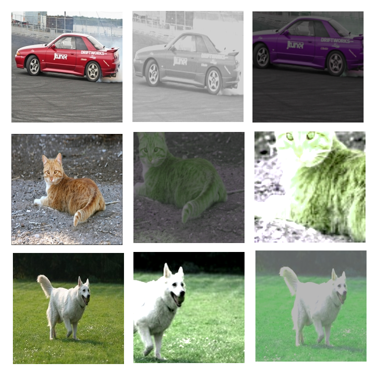
- For a given image, perform an image augmentation \(random crop, resize, color distortion etc...\)
- Positive pairs are defined as pairs of augmented images that came from the same original image
- Negative pairs are all other pairs that are not coming from the same image.
- In the example below, the black and white car and purple car are positive, while dog and cat are negative.
- Use a loss function that compares similarity between each pair of images in the batch.
The loss function, known as contrastive loss (CL), is based on the assumption that representations of images from the positive pairs are close, while the negative pairs representations are far away from each other. Common approaches of SSRL rely on numerous image pairs comparisons which require significant computational resources and are not practical on very large datasets. One way to solve this problem is to reduce the number of image comparisons to a fixed number of random images.
Another way to overcome this problem is to use a new SSRL approach named SwaV, which is a synergy of the following ideas:
- Enforce similar images to be part of the same cluster in the features space, so images can be assigned to a cluster instead of an explicit comparison between each pair of images. In other words, the idea is to train an embedding with consistent cluster assignments between augmentations of the same image. Intuitively we want to find clusters so that all views and transformations of the same image (like crops, color distortion etc...) will end up in the same cluster(more on this later).
- Multicrop data augmentation that allows to significantly increase the number of image comparisons without having a large increase of the memory and computational resources.
How multicrop works?
- Start with “standard” crops: crop x_c1 and x_c2 of image X.
- Take smaller crops from x_c1 and x_c2 in several smaller resolutions.
- Build positive examples from these crops.

More about SwaV and its Loss function :
- First we elaborate on the SwaV training scheme.
- For every image X in the batch:
- Create a number of augmentations.
- Create different positive pairs from these augmentations.
- Map the augmented images to their representations, z, using ResNet or other ConvNet.
- Define K cluster vectors C_1,...C_k ( C_1,..C_k are considered centroids of the clusters).
- For every positive pair of vector representations Z_t and Z_s build “code” vectors q_t and q_s.
- The code vectors q are vectors that describe the probabilities of “belonging” to the clusters (prototypes) {c_1,...,c_k} - the level of “closeness” to each cluster.
- Use the loss function L(Z_t, Z_s) to vectors Z_t and Z_s with the code vectors q_s and q_t.

How is the loss function defined?
$$\mathbf{L}(\mathbf{z_t, z_s}) = \mathit{l} \left(\mathbf{z_t}, \mathbf{q_s} \right) + \mathit{l} \left(\mathbf{z_s}, \mathbf{q_t} \right)$$
The loss is the sum of “swapped” similarity between the images representations Zt and Zs and their cluster assignments qt and qs.
Intuitively this means that we can predict the cluster of one version of an image from its other version, since if 2 vector versions (augmentations) of the same image capture the same information, it should be possible to predict the cluster of one vector from its similar vector.
I recommend watching this amazing animation by FAIR describing the SwaV process.
A bit on the mathematics:
$\mathit{l} \left(\mathbf{z_t}, \mathbf{q_s} \right)$ measures a similarity between feature vector zt and code vector qs.
This is a cross-entropy loss between 2 vectors: qs and pt:
$\mathit{l} \left(\mathbf{z_t}, \mathbf{q_s} \right) = - \sum_{k} \mathbf{q_s^{(k)}} \log{p_t^{(k)}} $
Where P_t is a softmax similarity vector that represents the distance of vector Z_t from each one of the clusters C_i. tau, is a temperature parameter.
$\mathbf{P_t^{(k)}} = \frac{\exp(\frac{1}{T}Z_t^Tc_k)}{\sum_{k'}\exp(\frac{1}{T}Z_t^Tc_{k'})}$
Then we sum the loss over all N images and over set T of the used augmentations, and obtain:
$-\frac{1}{N}\sum^N_{n=1}\sum_{s,t \sim \tau} \left[ \frac{1}{T} Z^T_{nt}Cq_{ns} - \log\sum^k_{k=1} \exp \left( \frac{z_{nt}^TC_k}{\tau}\right) - \log \sum^k_{k=1} \exp \left( \frac{Z^T_{ns}C_k}{\tau} \right) \right]$
This loss is jointly minimized with respect to the cluster prototypes C and the network weights used to produce the z vectors.
How is the clusters assignment done?
The goal is to assign B features vectors to K cluster vectors:


This means that we want to find mappings between the samples and the clusters. These mapping are called codes, and are represented by the matrix Q. In the case, when each sample is assigned to one cluster, these Q codes are basically 1-hot vectors.
So basically, we need a way of taking this batch of features vectors and then efficiently sending them to the different clusters (prototypes). This is an optimization problem similar to the well-known optimal transport problem which can be used, for example, to estimate similarity between domains. This problem is solved with Sinkhorn Knopp Algorithm.
Intuition on the solution to the cluster assignment problem:
We need to find the criterion of how to assign each feature vector to a cluster. In order to do so, the paper used a cost matrix, which is given by the dot product between the transposed clusters matrix and the matrix made up of Z vectors. This cost matrix represents the cost that we are going to pay when assigning a certain sample to a cluster. The goal is to minimize this cost.

Based on this cost matrix (see example below), when taking the sample Z_n, there is a very high cost when it is assigned to cluster 1 (marked in red), and a very low cost when it is assigned to the clusters k and K.

This problem can be turned into an optimization problem in the following way: optimize Q to maximize the similarity between features and the cluster vectors.
$\max_{Q\in{\mathcal{Q}}} Tr (Q^TC^TZ) + \epsilon H(Q)$
$H(Q) = - \sum_{ij}Q_{ij}\log{Q_{ij}}$ H defines the entropy of the Q matrix, is a regularization parameter.
Some intuition on the H regularization:
The term is a negative summation of entropy of each of the elements qij in the matrix.
Since 0<=qij <=1 , the term $\sum q_{ij} \log(q_{ij})$ is positive. In order to maximize it, q will be somewhere in the middle between 0 to 1. So basically the regularization term helps to avoid trivial solutions (all vectors belong to the same cluster with a high probability)
Solution to the above problem is given by:
$Q^* = Diag(u) \exp \left( \frac{C^TZ}{\epsilon} \right) Diag(v)_t$
Avoiding the trivial solution:
In order to avoid the trivial solution where all features vectors are assigned to the same one cluster, a constraint is added: all clusters(prototypes) are selected the same amount of times. The code’s equipartition constraint is represented by this set:
$Q = \left Q \in \mathbb{R_+^{K \times B}} | Q1_B = \frac{1}{K}1_K,Q^T1_K = \frac{1}{B}1_B \right$
1K denotes the vector of ones of dimension K. This constraint enforces that on average each cluster is selected at least B/K times in the batch.
Results and achievements of this paper:
It was shown that SwaV produces better vector representations than other SSRL methods. The comparison is done in a standard way:
Train network (usually resnet) in a self supervised way and in a supervised way on ImageNet.
Freeze weights and add a linear layer on top of the network.
Test the above on different datasets and different downstream tasks like classification or object segmentation.
Some of the results:

- SwaV representations outperforms supervised representation:A comparison of different datasets for both classification measured in top 1 accuracy), and object detection (measured as mean avg. precision) tasks.
- SwaV outperforms other self supervised methods:

There are several other interesting experiments that you are encouraged to read in this paper
Final words
If you want to learn about SSRL techniques and enjoy great insights, then you should definitely read this paper. Also, they did a lot of work testing SwaV on different tasks and datasets, and provided the code.
#deepnightlearners
Rachel Shalom is a senior Data scientist at Dell with previous experience as a DS in healthcare startups. She holds a B.Sc. in Mathematics, an MBA, and she graduated Yandex School of Advanced Machine Learning.


